TikZ Tutorial for Math Teachers: Drawing Precise Geometry

TikZ is a LaTeX package for drawing vector graphics directly from code. Unlike pasting images from other applications, TikZ drawings offer:

• High precision — coordinates are written as numbers, so dimensions are always exact;
• Consistency — fonts and drawing styles blend seamlessly with your document;
• Easy to modify — just edit numbers, no need to redraw;
• Free — already available on Overleaf with no extra installation.

Getting Started on Overleaf

Just add two lines to your preamble (the part before \begin{document}):

\usepackage{tikz}
\usetikzlibrary{arrows.meta, calc, quotes, backgrounds}

The first line loads the TikZ package. The second loads additional libraries — extra features like modern arrows, coordinate calculations, and labels. Only load the libraries you need to keep compilation fast.

TikZ Basics

Points and Lines

TikZ uses the Cartesian coordinate system: (x,y). Points are drawn with \filldraw, lines with \draw.

\begin{tikzpicture}
  % Points at coordinates (1,2) and (4,3)
  \filldraw[blue] (1,2) circle (3pt);
  \filldraw[red]  (4,3) circle (3pt);
  % Line from the first point to the second
  \draw[thick] (1,2) -- (4,3);
\end{tikzpicture}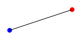

Colors, Line Thickness, and Styles

\draw[red]         (0,0) -- (2,0);   % thin red line
\draw[blue, thick] (0,1) -- (2,1);   % thick blue line
\draw[dashed]      (0,2) -- (2,2);   % dashed
\draw[dotted]      (0,3) -- (2,3);   % dotted
\draw[->]          (0,4) -- (2,4);   % arrow to the right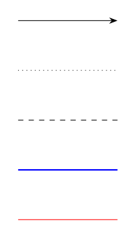

Adding Labels (Nodes)

A node is text attached to a specific point. Label position is set with above, below, left, right, etc.

\draw (0,0) -- (3,0);
\node[above] at (1.5,0) {center};
\node[below left] at (0,0) {bottom left};
\node[below right] at (3,0) {bottom right};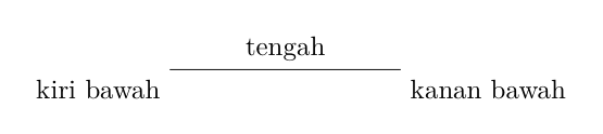

Case Study 1: The Cartesian Plane

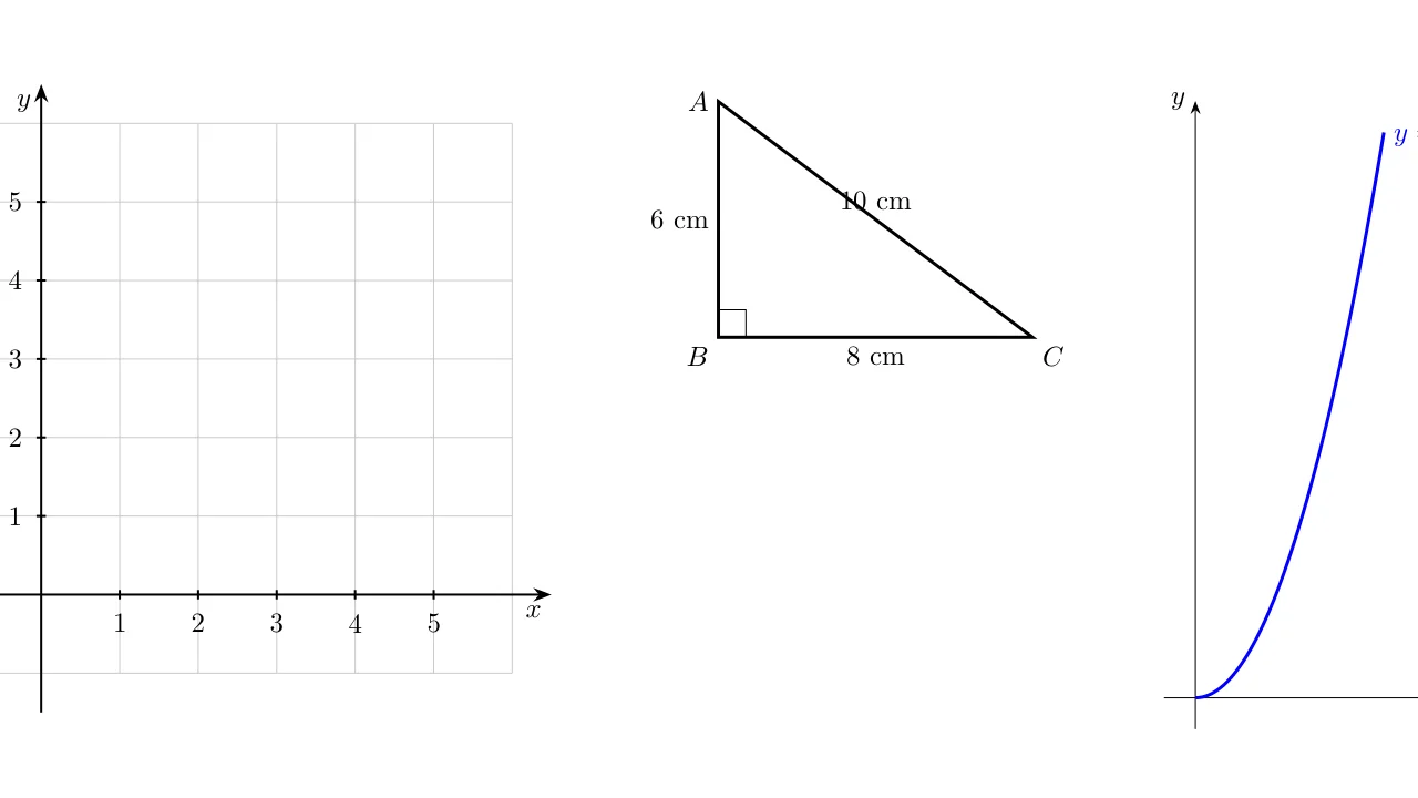
A classic example: a Cartesian plane with axes, arrows, grid, and number scale.

\begin{tikzpicture}[>=Stealth]
  % grid
  \draw[gray!40] (-1,-1) grid (6,6);
  % axes
  \draw[->, thick] (-1.5,0) -- (6.5,0) node[below left] {$x$};
  \draw[->, thick] (0,-1.5) -- (0,6.5) node[below left] {$y$};
  % scale
  \foreach \n in {1,...,5}{
    \draw[thick] (\n,0.06) -- (\n,-0.06);
    \node[below] at (\n,-0.12) {\n};
    \draw[thick] (0.06,\n) -- (-0.06,\n);
    \node[left] at (-0.12,\n) {\n};
  }
\end{tikzpicture}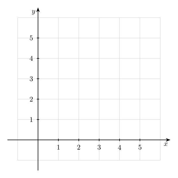

Tip: the \foreach command is a loop — a concise way to repeat a command with different values. It is very useful for scales and grids.

Case Study 2: The Pythagorean Right Triangle

Combine all concepts: points, lines, colors, labels, and the right-angle symbol.

\begin{tikzpicture}[>=Stealth]
  % vertices: B at (0,0), A above, C to the right
  \coordinate (A) at (0,3);
  \coordinate (B) at (0,0);
  \coordinate (C) at (4,0);

  % triangle sides
  \draw[very thick] (A) -- (B) -- (C) -- cycle;

  % right-angle symbol at B
  \draw (0.35,0) -- (0.35,0.35) -- (0,0.35);

  % vertex labels
  \node[left] at (A) {$A$};
  \node[below left] at (B) {$B$};
  \node[below right] at (C) {$C$};

  % side length labels
  \node[left] at (0,1.5) {$6$ cm};
  \node[below] at (2,0) {$8$ cm};
  \node[above, sloped] at ($(A)!0.5!(C)$) {$10$ cm};
\end{tikzpicture}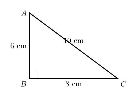

Note: \coordinate names a point so it can be reused easily. The expression $(A)!0.5!(C)$ computes the midpoint between $A$ and $C$ — a feature of the calc library.

Case Study 3: Function Graphs

TikZ can also draw function graphs with \draw plot.

\begin{tikzpicture}[>=Stealth, scale=0.8]
  % axes
  \draw[->] (-0.5,0) -- (4.5,0) node[below] {$x$};
  \draw[->] (0,-0.5) -- (0,9.5) node[left] {$y$};

  % graph of y = x^2 from x=0 to x=3
  \draw[blue, very thick, domain=0:3, samples=60]
       plot (\x, {\x*\x});

  % label
  \node[blue, right] at (3,9) {$y = x^2$};
\end{tikzpicture}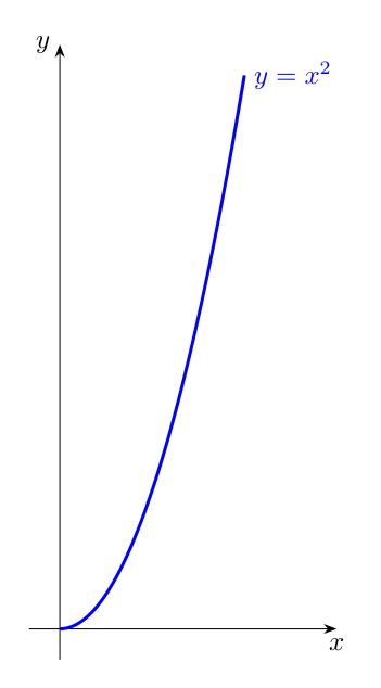

Tip: domain=0:3 limits the $x$ range, samples=60 sets the number of computed points — the higher the number, the smoother the curve.

Case Study 4: Dark Theme

For presentations or on-screen teaching media, a dark theme can be more comfortable to read.

\usetikzlibrary{backgrounds} % in the preamble

\begin{tikzpicture}[
    background rectangle/.style={fill=black!95},
    show background rectangle,
    every node/.style={text=white},
  ]
  % dark grid
  \draw[gray!40] (-0.5,-0.5) grid (4.5,4.5);
  % white axes
  \draw[->, white, thick] (-1,0) -- (5,0);
  \draw[->, white, thick] (0,-1) -- (0,5);
  % cyan points
  \filldraw[cyan] (1,2) circle (3pt);
  \filldraw[cyan] (4,3) circle (3pt);
  \draw[cyan, thick] (1,2) -- (4,3);
\end{tikzpicture}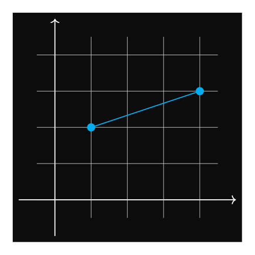

Quick Reference of Essential Commands

Conclusion

TikZ may look intimidating at first, but once you master five basic concepts — points, lines, nodes, colors, and foreach — you can draw almost any geometry for worksheets, exam questions, or presentation slides.

The key to practice: start small, compile often, and look at the results immediately. Overleaf shows output in real time, so the learning process feels fast.

References

• Official TikZ documentation: ctan.org/pkg/pgf
• Example gallery: texample.net
• LaTeX wiki: overleaf.com/learn
• Related article on this blog: Drawing a Rose Curve with TikZ