3D Spherical Polar Plots and Spherical Harmonics Visualization with tikz-3dplot

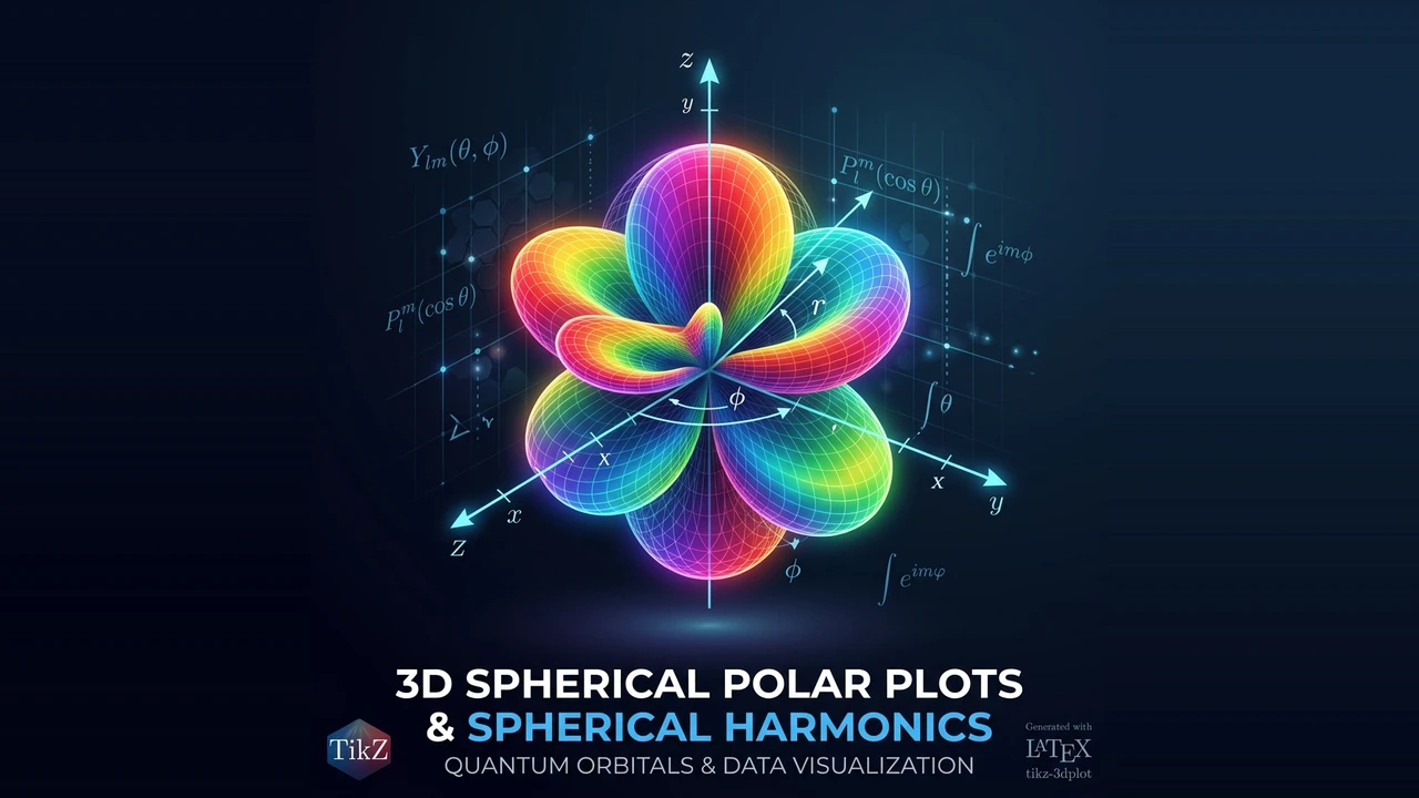
This article explores how to visualize 3D mathematical functions in spherical polar coordinates and Spherical Harmonics using the tikz-3dplot package in LaTeX.

Introduction

In quantum mechanics, geophysics, and mathematical physics, Spherical Harmonics $Y_l^m(\theta, \phi)$ represent a system of orthogonal functions that describe the angular dependence of wave equations in three-dimensional space. One of their most famous applications is representing atomic electron orbitals ($s, p, d, f$) in hydrogen-like atoms.

Rendering accurate 3D plots showing both the magnitude and phase of spherical functions directly inside LaTeX was once a challenging task. However, Jeff Hein authored an extension for the tikz-3dplot package that enables native 3D spherical polar surface plotting in TikZ.

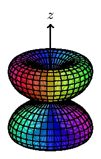
In these visualizations, the 3D geometric shape is defined by the function magnitude $r(\theta, \phi)$, while parametric color shading (hue) conveys the complex phase angle $\phi$.

LaTeX Source Code

Here is the complete LaTeX code by Jeff Hein to visualize the $Y_{2,1}(\theta, \phi)$ spherical harmonic function along with parameters for other quantum orbitals:

% harmonics.tex: produces spherical harmonic plots using the 3dplot package
% Author: Jeff Hein
\documentclass{minimal}
\usepackage{tikz}             % for TikZ graphics
\usepackage{tikz-3dplot}      % for 3dplot functionality
\usepackage[active,tightpage]{preview}
\PreviewEnvironment{tikzpicture}
\setlength\PreviewBorder{2mm}

\begin{document}

% Define 3D viewing angle (camera orientation: theta=70, phi=135)
\tdplotsetmaincoords{70}{135}

\begin{tikzpicture}[line join=bevel,tdplot_main_coords, fill opacity=.7]
  % Spherical surface plot for L=2, M_L=1
  \tdplotsphericalsurfaceplot[parametricfill]{72}{36}%
    {sqrt(15/2)*sin(\tdplottheta)*cos(\tdplottheta)}{black}{\tdplotphi}%
    {\draw[color=black,thick,->] (0,0,0) -- (2,0,0) node[anchor=north east]{$x$};}%
    {\draw[color=black,thick,->] (0,0,0) -- (0,2,0) node[anchor=north west]{$y$};}%
    {\draw[color=black,thick,->] (0,0,0) -- (0,0,2) node[anchor=south]{$z$};}%
\end{tikzpicture}

\end{document}

Output Produced

Compiling the code above generates a beautiful 3D surface plot of the $Y_{2,1}$ orbital:

Detailed Code Analysis & tikz-3dplot Components

1. Setting Up 3D View Orientation

\tdplotsetmaincoords{70}{135}

This command specifies the elevation angle ($\theta = 70^\circ$) and azimuth angle ($\phi = 135^\circ$) for the 3D perspective projection. Option tdplot_main_coords is then passed to tikzpicture so all coordinates align with this camera view.

2. Syntax of \tdplotsphericalsurfaceplot

The primary command \tdplotsphericalsurfaceplot accepts several key arguments:

\tdplotsphericalsurfaceplot[options]{n_phi}{n_theta}{function_r}{line_color}{phase_function}{x_axis}{y_axis}{z_axis}

• [parametricfill]: Enables spectrum gradient coloring based on the phase angle variable $\phi$.
• {72}{36}: Defines the grid resolution (72 azimuthal steps for $\phi$ and 36 polar steps for $\theta$).
• {sqrt(15/2)*sin(\tdplottheta)*cos(\tdplottheta)}: The mathematical equation defining the radial distance $r(\theta, \phi)$.
• {\tdplotphi}: The function specifying the parametric hue variation.
• Cartesian Axes $(x,y,z)$: The final three arguments allow drawing coordinate axes directly inside the plot environment.

Gallery of Other Spherical Harmonics Equations

You can swap the $r(\theta, \phi)$ function expression to display various atomic orbital shapes:

1. $s$-Orbital ($L = 0, M_L = 0$)

Perfect spherical symmetry with constant radius:

{1}{black}{0}

2. $p_z$-Orbital ($L = 1, M_L = 0$)

Two vertical lobes oriented along the $z$-axis:

{sqrt(3)*cos(\tdplottheta)}{black}{0}

3. $p_{x,y}$-Orbital ($L = 1, M_L = \pm 1$)

Horizontal lobes along the $xy$-plane:

{sqrt(3/2)*sin(\tdplottheta)}{black}{\tdplotphi}

4. $d_{z^2}$-Orbital ($L = 2, M_L = 0$)

Two primary lobes along the $z$-axis with an equatorial doughnut torus:

{sqrt(5)/2*(3*cos(\tdplottheta)^2 - 1)}{black}{-\tdplotphi}

5. $f$-Orbital ($L = 3, M_L = 0$)

Complex multi-lobed structure:

{sqrt(7)/2*(5*cos(\tdplottheta)^3 - 3*cos(\tdplottheta))}{black}{0}

TikZ Experimentation

Try these modifications to customize your plot:

1. Adjust Surface Opacity: Change fill opacity=.7 to .9 for a solid surface or .4 to reveal internal grid lines.
2. Modify Camera Perspective: Change \tdplotsetmaincoords{60}{45} to view the surface from top or side angles.

Conclusion

The tikz-3dplot package offers an elegant solution for rendering 3D spherical polar surface plots directly inside LaTeX without depending on external software like MATLAB or Python. Its parametric color fill capabilities make intuitive visualization of complex functions and quantum wave functions effortless.

References

1. Jeff Hein, Spherical polar plots with 3dplot, TeXample.net
2. Jeff Hein, Documentation for the 3dplot.sty package, 3dplot Manual
3. Wikipedia, Spherical Harmonics, en.wikipedia.org/wiki/Spherical_harmonics

Written by: Aan Triono
License: CC BY-SA 4.0