Drawing Nested Rotated Polygons and Spiral Patterns with TikZ in LaTeX

Aan Triono included in category LaTeX

2026-07-18 2026-08-08 702 words 4 minutes

A detailed analysis of creating spiral optical illusion patterns with nested rotated polygons (hexagon, pentagon, square) using loops and color gradients in LaTeX TikZ.

Contents

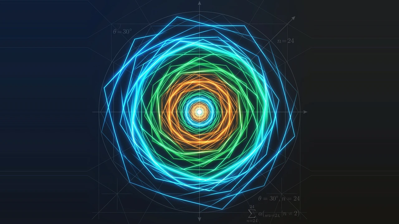
This article explores how to draw nested rotated polygon spiral patterns (op-art optical illusions) using loops and color gradients in LaTeX TikZ.

Introduction

One of the most striking visual effects in fractal geometry and optical art (op-art) is the spiral pattern created by recursively nesting polygons.

When a polygon is progressively rotated by a fraction of an angle and scaled down toward the center, our eyes perceive a deep 3D optical vortex.

This article explores a TikZ implementation by Dr. rer. nat. Ismael Gutierrez Garcia (extending Alain Matthes’ rotated triangle concept). We will break down how a simple \foreach loop, relative coordinate positioning with pos=.10, and progressive color density scaling produce mesmerizing hexagon, pentagon, and square spiral structures.

LaTeX Source Code

Here is the complete LaTeX code to generate the three rotated polygon variations:

% Rotated polygons
% Author: Dr. rer. nat. Ismael Gutierrez Garcia
\documentclass{article}
\usepackage[usenames,dvipsnames,pdftex]{xcolor}
\usepackage{tikz}
\usepackage[active,tightpage]{preview}
\PreviewEnvironment{tikzpicture}
\setlength\PreviewBorder{5pt}%
\usepackage{ifthen}

\begin{document}

% -------------------------------------------------------------
% 1. ROTATED HEXAGON (BlueGreen)
% -------------------------------------------------------------
\newcounter{density}
\setcounter{density}{20}

\begin{tikzpicture}
  \def\couleur{BlueGreen}
  
  % Initial Vertex Position Setup for Hexagon
  \path[coordinate] (0,0) coordinate(A)
    ++( 120:6cm) coordinate(B)
    ++( 60:6cm) coordinate(C)
    ++(  0:6cm) coordinate(D)
    ++(-60:6cm) coordinate(E)
    ++(240:6cm) coordinate(F);
    
  \draw[fill=\couleur!\thedensity] (A) -- (B) -- (C) --(D) -- (E) -- (F)-- cycle;

  % 40-Step Loop for Rotation & Scaling
  \foreach \x in {1,...,40}{
    \pgfmathsetcounter{density}{\thedensity+10}
    \setcounter{density}{\thedensity}
    
    \path[coordinate] coordinate(X) at (A){};
    \path[coordinate]
      (A) -- (B) coordinate[pos=.10](A)
      -- (C) coordinate[pos=.10](B)
      -- (D) coordinate[pos=.10](C)
      -- (E) coordinate[pos=.10](D)
      -- (F) coordinate[pos=.10](E)
      -- (X) coordinate[pos=.10](F);
      
    \draw[fill=\couleur!\thedensity] (A)--(B)--(C)--(D)--(E)--(F)--cycle;
  }
\end{tikzpicture}

% -------------------------------------------------------------
% 2. ROTATED PENTAGON (LimeGreen)
% -------------------------------------------------------------
\setcounter{density}{20}

\begin{tikzpicture}
  \def\couleur{LimeGreen}
  
  \path[coordinate] (0,0) coordinate(A)
    ++( 144:10cm) coordinate(B)
    ++( 72:10cm) coordinate(C)
    ++(  0:10cm) coordinate(D)
    ++(-72:10cm) coordinate(E);
    
  \draw[fill=\couleur!\thedensity] (A) -- (B) -- (C) --(D) -- (E) -- cycle;

  \foreach \x in {1,...,40}{
    \pgfmathsetcounter{density}{\thedensity+10}
    \setcounter{density}{\thedensity}
    
    \path[coordinate] coordinate(X) at (A){};
    \path[coordinate]
      (A) -- (B) coordinate[pos=.10](A)
      -- (C) coordinate[pos=.10](B)
      -- (D) coordinate[pos=.10](C)
      -- (E) coordinate[pos=.10](D)
      -- (X) coordinate[pos=.10](E);
      
    \draw[fill=\couleur!\thedensity] (A)--(B)--(C)--(D)--(E)--cycle;
  }
\end{tikzpicture}

% -------------------------------------------------------------
% 3. ROTATED SQUARE (OrangeRed)
% -------------------------------------------------------------
\setcounter{density}{20}

\begin{tikzpicture}
  \def\couleur{OrangeRed}
  
  \path[coordinate] (0,0) coordinate(A)
    ++( 90:12cm) coordinate(B)
    ++(  0:12cm) coordinate(C)
    ++(-90:12cm) coordinate(D);
    
  \draw[fill=\couleur!\thedensity] (A) -- (B) -- (C) --(D) -- cycle;

  \foreach \x in {1,...,40}{
    \pgfmathsetcounter{density}{\thedensity+20}
    \setcounter{density}{\thedensity}
    
    \path[coordinate] coordinate(X) at (A){};
    \path[coordinate]
      (A) -- (B) coordinate[pos=.10](A)
      -- (C) coordinate[pos=.10](B)
      -- (D) coordinate[pos=.10](C)
      -- (X) coordinate[pos=.10](D);
      
    \draw[fill=\couleur!\thedensity] (A)--(B)--(C)--(D)--cycle;
  }
\end{tikzpicture}

\end{document}

Output Produced

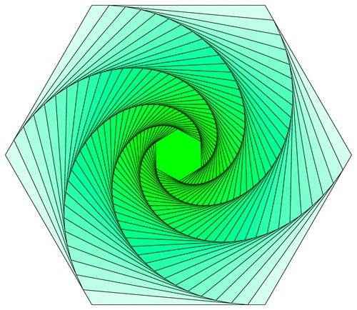
The resulting graphical output displays three polygon variations with vibrant color depth and rotation:

Detailed Code Structure Analysis

1. Constructing Initial Polygons via Polar Vectors

Vertex coordinates start at the origin (0,0) and connect sequentially using polar vector shifts ++(angle:distance):

Hexagon (6-gon): Uses $60^\circ$ angular increments (120:6cm, 60:6cm, 0:6cm, -60:6cm, 240:6cm).
Pentagon (5-gon): Uses $72^\circ$ angular increments (144:10cm, 72:10cm, 0:10cm, -72:10cm).
Square (4-gon): Uses $90^\circ$ angular increments (90:12cm, 0:12cm, -90:12cm).

2. Vertex Update Algorithm `pos=.10`

The magic behind the automatic rotation and scaling lies in these lines:

\path[coordinate] coordinate(X) at (A){};
\path[coordinate] (A) -- (B) coordinate[pos=.10](A)
                  -- (C) coordinate[pos=.10](B) ...

Variable X holds the original location of vertex $A$ before it is overwritten.
Option pos=.10 picks the point located at $10\%$ along the edge from $A$ to $B$ , and assigns it as the new position for vertex $A$ .
Because every vertex shifts $10\%$ toward its neighbor cyclically, connecting the new vertices creates a polygon that is both rotated and shrunk.

3. Color Density Gradients (`density`)

On each loop iteration, the density counter increases:

\pgfmathsetcounter{density}{\thedensity+10}
\draw[fill=\couleur!\thedensity] (A)--(B)...;

Expression BlueGreen!20 fills the outermost polygon with 20% BlueGreen and 80% white.
As iterations approach the center, color saturation increases (30%, 40%, 50%, …), yielding a 3D depth gradient effect.

TikZ Experimentation

Try these modifications to explore further:

Varying Rotation Speed (pos): Change pos=.10 to pos=.05 for tighter rotations with more layers, or pos=.20 for sharper twists.
Increasing Loop Iterations: Extend \foreach \x in {1,...,40} to 1,...,60 to spiral all the way down to the central point.
Custom Color Schemes: Experiment with other xcolor palettes such as RoyalBlue, PurplishRed, or Goldenrod.

Conclusion

Dr. Ismael Gutierrez Garcia’s code demonstrates how concise iterative algorithms in TikZ can produce captivating results. By combining position interpolation (pos=.10) with dynamic color saturation, TikZ transforms basic geometry into stunning fractal art.

References

Ismael Gutierrez Garcia, Rotated polygons, TeXample.net
Alain Matthes, Rotated triangle, TeXample.net
Till Tantau, The TikZ and PGF Manual, v3.1.10, 2024.

Written by: Aan Triono
License: CC BY-SA 4.0

Contents

Drawing Nested Rotated Polygons and Spiral Patterns with TikZ in LaTeX

Introduction

LaTeX Source Code

Output Produced

Detailed Code Structure Analysis

1. Constructing Initial Polygons via Polar Vectors

2. Vertex Update Algorithm pos=.10

3. Color Density Gradients (density)

TikZ Experimentation

Conclusion

References

Related Content

3D Spherical Polar Plots and Spherical Harmonics Visualization with tikz-3dplot

Calculating C(n,4) Intersection Points of Chords in a Circle with TikZ

Creating a 2026 Circular Year Calendar using the TikZ Calendar Library in LaTeX

Drawing a Directed Complete Graph (K16) with TikZ in LaTeX

Drawing a Sunflower Pattern (Phyllotaxis) with TikZ in LaTeX

2. Vertex Update Algorithm `pos=.10`

3. Color Density Gradients (`density`)