Perigal's Dissection: A Geometric Proof of the Pythagorean Theorem in LaTeX
The Pythagorean theorem is one of the most famous fundamental principles in mathematics. There are many ways to prove it, both algebraically and geometrically. One of the most elegant and visual geometric proofs is Perigal’s Dissection, discovered by Henry Perigal in 1873.
In this article, we will learn how to create a visualization of Perigal’s Dissection using the TikZ package in LaTeX.
Introduction
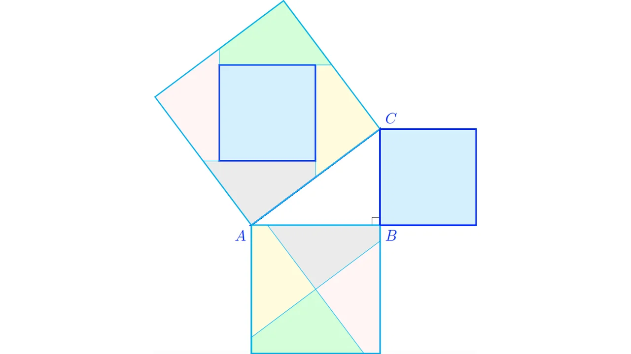
Perigal’s dissection is a method for proving the Pythagorean theorem () by cutting (dissecting) the square constructed on the longer leg of a right-angled triangle into four congruent parts.
These cuts are made by drawing two perpendicular lines passing through the center of the square, where one of the lines is parallel to the hypotenuse of the triangle.
These four parts, along with the intact square of the shorter leg, can be rearranged perfectly to cover the entire area of the square constructed on the hypotenuse.
Complete LaTeX Code
Here is the complete LaTeX code using the TikZ library (intersections and math) to generate the Perigal’s dissection diagram precisely:
\documentclass{article}
\usepackage{tikz}
\usetikzlibrary{intersections}
\usetikzlibrary{math}
\usepackage[active,tightpage]{preview}
\PreviewEnvironment{tikzpicture}
\setlength\PreviewBorder{0.125pt}

% File name: perigals-dissection.tex
% Description: A geometric proof of the Pythagorean theorem using Perigal's dissection.
% Author: Efraín Soto Apolinar.

\begin{document}
\begin{tikzpicture}[scale=0.75]
\tikzmath{function rotacionx(\x,\y,\angulo) {return \x*cos(\angulo) + \y*sin(\angulo);};}
\tikzmath{function rotaciony(\x,\y,\angulo) {return -\x*sin(\angulo) + \y*cos(\angulo);};}
\pgfmathsetmacro{\dx}{0.25}

% Vertices of the right triangle
\pgfmathsetmacro{\Ax}{0}
\pgfmathsetmacro{\Ay}{0}
\coordinate (A) at (\Ax,\Ay);
\pgfmathsetmacro{\Bx}{4}
\pgfmathsetmacro{\By}{0}
\coordinate (B) at (\Bx,\By);
\pgfmathsetmacro{\Cx}{4}
\pgfmathsetmacro{\Cy}{3}
\coordinate (C) at (\Cx,\Cy);

% Lengths of the sides
\pgfmathsetmacro{\lAB}{sqrt((\Bx - \Ax)*(\Bx - \Ax) + (\By - \Ay)*(\By - \Ay))}
\pgfmathsetmacro{\lAC}{sqrt((\Cx - \Ax)*(\Cx - \Ax) + (\Cy - \Ay)*(\Cy - \Ay))}
\pgfmathsetmacro{\lBC}{sqrt((\Cx - \Bx)*(\Cx - \Bx) + (\Cy - \By)*(\Cy - \By))}

% Slopes of the sides of the triangle
\pgfmathsetmacro{\mAC}{(\Cy - \Ay)/(\Cx - \Ax)}
\pgfmathsetmacro{\mAB}{(\By - \Ay)/(\Bx - \Ax)}

\pgfmathsetmacro{\angA}{atan(\mAC)}
\pgfmathsetmacro{\angB}{90.0}
\pgfmathsetmacro{\angC}{90.0-\angA}
\pgfmathsetmacro{\angAH}{45+\angA}

% Coordinates of the vertices of the squares on the sides
\pgfmathsetmacro{\Dx}{0}
\pgfmathsetmacro{\Dy}{-\lAB}
\coordinate (D) at (\Dx,\Dy);
\pgfmathsetmacro{\Ex}{\Bx}
\pgfmathsetmacro{\Ey}{-\lAB}
\coordinate (E) at (\Ex,\Ey);
\pgfmathsetmacro{\Fx}{\Bx+\lBC}
\pgfmathsetmacro{\Fy}{0}
\coordinate (F) at (\Fx,\Fy);
\pgfmathsetmacro{\Gx}{\Bx+\lBC}
\pgfmathsetmacro{\Gy}{\lBC}
\coordinate (G) at (\Gx,\Gy);
\pgfmathsetmacro{\Hx}{sqrt(2.0)*\lAC*cos(45+\angA)}
\pgfmathsetmacro{\Hy}{sqrt(2.0)*\lAC*sin(45+\angA)}
\coordinate (H) at (\Hx,\Hy);
\pgfmathsetmacro{\Ix}{rotacionx(\Cx,\Cy,-90)}
\pgfmathsetmacro{\Iy}{rotaciony(\Cx,\Cy,-90)}
\coordinate (I) at (\Ix,\Iy);

% Coordinates of the centroid of the square upon the hypotenuse
\pgfmathsetmacro{\Mx}{0.5*(\Ax+\Hx)}
\pgfmathsetmacro{\My}{0.5*(\Ay+\Hy)}
\coordinate (M) at (\Mx,\My);

% Points upon the hypotenuse to draw the dissection
\pgfmathsetmacro{\Jx}{\Mx+0.5*\lBC}
\pgfmathsetmacro{\Jy}{\My+0.5*\lBC}
\coordinate (J) at (\Jx,\Jy);
\pgfmathsetmacro{\Kx}{\Mx-0.5*\lBC}
\pgfmathsetmacro{\Ky}{\My+0.5*\lBC}
\coordinate (K) at (\Kx,\Ky);
\pgfmathsetmacro{\Lx}{\Mx-0.5*\lBC}
\pgfmathsetmacro{\Ly}{\My-0.5*\lBC}
\coordinate (L) at (\Lx,\Ly);
\pgfmathsetmacro{\Nx}{\Mx+0.5*\lBC}
\pgfmathsetmacro{\Ny}{\My-0.5*\lBC}
\coordinate (N) at (\Nx,\Ny);

% Length for dissection
\pgfmathsetmacro{\mCH}{(\Hy - \Cy)/(\Hx - \Cx)}
\pgfmathsetmacro{\xp}{\Cx+(\Jy-\Cy)/\mCH}
\pgfmathsetmacro{\yp}{\Jy}
\pgfmathsetmacro{\ld}{sqrt((\Jx - \xp)*(\Jx - \xp) + (\Jy - \yp) * (\Jy - \yp))}

% Vertices of the dissection upon the longer leg (AB)
\pgfmathsetmacro{\Cunox}{\Bx}
\pgfmathsetmacro{\Cunoy}{\By - \ld}
\coordinate (Cuno) at (\Cunox,\Cunoy);
\pgfmathsetmacro{\Cdosx}{\Ax + \ld}
\pgfmathsetmacro{\Cdosy}{\Ay}
\coordinate (Cdos) at (\Cdosx,\Cdosy);
\pgfmathsetmacro{\Ctresx}{\Dx}
\pgfmathsetmacro{\Ctresy}{\Dy + \ld}
\coordinate (Ctres) at (\Ctresx,\Ctresy);
\pgfmathsetmacro{\Ccuatrox}{\Ex - \ld}
\pgfmathsetmacro{\Ccuatroy}{\Ey}
\coordinate (Ccuatro) at (\Ccuatrox,\Ccuatroy);

\path[name path=UT] (Cuno) -- (Ctres);
\path[name path=DC] (Cdos) -- (Ccuatro);
\path[name intersections={of=UT and DC}];
\coordinate (Q) at (intersection-1);

\pgfmathsetmacro{\ejex}{max(\Ax,\Bx,\Cx) + 1.0}
\pgfmathsetmacro{\ejey}{max(\Ay,\By,\Cy) + 1.0}

% The right triangle
\draw[black] (\Bx-\dx,0) -- (\Bx-\dx,\dx) -- (\Bx,\dx);
\draw[blue,thick] (A) -- (B) -- (C) -- cycle;
\fill[blue] (A) circle (1.0pt) node[below left]{$A$};
\fill[blue] (B) circle (1.0pt) node[below right]{$B$};
\fill[blue] (C) circle (1.0pt) node[above right]{$C$};

% Squares on the sides of the right triangle
\draw[cyan,thick] (0,0) rectangle (\lAB,-\lAB); % Side AB (longer leg)
\draw[cyan,thick,rotate=\angA] (0,0) rectangle (\lAC,\lAC); % Side AC (hypotenuse)
\draw[blue,thick,fill=cyan!15,shift={(\Bx,\By)}] (0,0) rectangle (\lBC,\lBC); % Side BC (shorter leg)

% Rectangle of dissection
\draw[blue,thick,fill=cyan!15] (J) -- (K) -- (L) -- (N) -- (J);

% Compute the intersections to draw the dissection
\coordinate (Jp) at (\Jx+2.0,\Jy);
\path[name path=CH] (C) -- (H);
\path[name path=JJp] (J) -- (Jp);
\path[name intersections={of=CH and JJp}];
\coordinate (Huno) at (intersection-1);

\coordinate (Np) at (\Nx,\Ny-2.0);
\path[name path=AC] (A) -- (C);
\path[name path=NNp] (N) -- (Np);
\path[name intersections={of=AC and NNp}];
\coordinate (Hdos) at (intersection-1);

\coordinate (Lp) at (\Lx-2.0,\Ly);
\path[name path=AI] (A) -- (I);
\path[name path=LLp] (L) -- (Lp);
\path[name intersections={of=AI and LLp}];
\coordinate (Htres) at (intersection-1);

\coordinate (Kp) at (\Kx,\Ky+2.0);
\path[name path=HI] (H) -- (I);
\path[name path=KKp] (K) -- (Kp);
\path[name intersections={of=HI and KKp}];
\coordinate (Hcuatro) at (intersection-1);

% Disection upon the hypotenuse
\draw[cyan,fill=yellow!35,opacity=0.5] (C) -- (Huno) -- (J) -- (Hdos) -- cycle;
\draw[cyan,fill=gray!35,opacity=0.5] (A) -- (Hdos) -- (N) -- (Htres) -- cycle;
\draw[cyan,fill=pink!35,opacity=0.5] (I) -- (Htres) -- (L) -- (Hcuatro) -- cycle;
\draw[cyan,fill=green!35,opacity=0.5] (H) -- (Huno) -- (K) -- (Hcuatro) -- cycle;

% Disection upon the longest leg (AB)
\draw[cyan,fill=gray!35,opacity=0.5] (Q) -- (Cuno) -- (B) -- (Cdos) -- cycle;
\draw[cyan,fill=yellow!35,opacity=0.5] (Q) -- (Cdos) -- (A) -- (Ctres) -- cycle;
\draw[cyan,fill=green!35,opacity=0.5] (Q) -- (Ctres) -- (D) -- (Ccuatro) -- cycle;
\draw[cyan,fill=pink!35,opacity=0.5] (Q) -- (Ccuatro) -- (E) -- (Cuno) -- cycle;

\end{tikzpicture}
\end{document}
The output of the code is as follows:
Detailed Code Explanation
Let’s analyze the mathematical concepts and main TikZ commands used in the code above:
1. Custom Coordinate Rotation (\tikzmath)
To calculate geometric rotation positions, custom functions were defined using the math library:
\tikzmath{function rotacionx(\x,\y,\angulo) {return \x*cos(\angulo) + \y*sin(\angulo);};}
\tikzmath{function rotaciony(\x,\y,\angulo) {return -\x*sin(\angulo) + \y*cos(\angulo);};}
The rotacionx and rotaciony functions calculate the new and coordinates after rotating a point by \angulo degrees. This is essential for precisely aligning the square on the inclined hypotenuse.
2. Parameterization Using PGF (\pgfmathsetmacro)
Geometric constants such as the side lengths of the right triangle (, , hypotenuse ), the slope angle of the hypotenuse (\angA), and the center coordinates of the dissection are computed dynamically using \pgfmathsetmacro. This ensures the diagram is precise and scalable.
3. Path Intersections (intersections)
The cutting lines of the dissection are computed using the intersections library. TikZ automatically detects the meeting point between two pathways:
\path[name path=UT] (Cuno) -- (Ctres);
\path[name path=DC] (Cdos) -- (Ccuatro);
\path[name intersections={of=UT and DC}];
\coordinate (Q) at (intersection-1);
This line detects the intersection point Q, which serves as the centroid of the dissection cuts on square (the longer leg).
4. Coloring the Geometrical Pieces
Each dissection slice is colored with a different fill (yellow, gray, pink, green) at half transparency (opacity=0.5) to help readers visually trace how the pieces from the bottom square () can be rearranged to fit perfectly into the square on the hypotenuse.
The square on the shorter leg () is filled with light blue (cyan!15) and is positioned in the center of the hypotenuse square as the fifth compiling piece.
How to Compile the Document
To compile the LaTeX file:
- Ensure a LaTeX environment (such as TeX Live, MiKTeX, or Overleaf) is installed.
- Copy the LaTeX code above into a new file named
perigals-dissection.tex. - Compile using pdfLaTeX or XeLaTeX.
- The
previewpackage will crop the output PDF page precisely to fit the boundaries of the TikZ picture.
Conclusion
Perigal’s dissection provides a visually striking proof of the Pythagorean theorem without requiring complex algebraic formulas. With the help of the math and intersections libraries in TikZ, we can create precise and elegant representations of classical geometry theorems. Happy TeXing!