Pascal's Triangle: Computation and Hexagonal Visualization in LaTeX

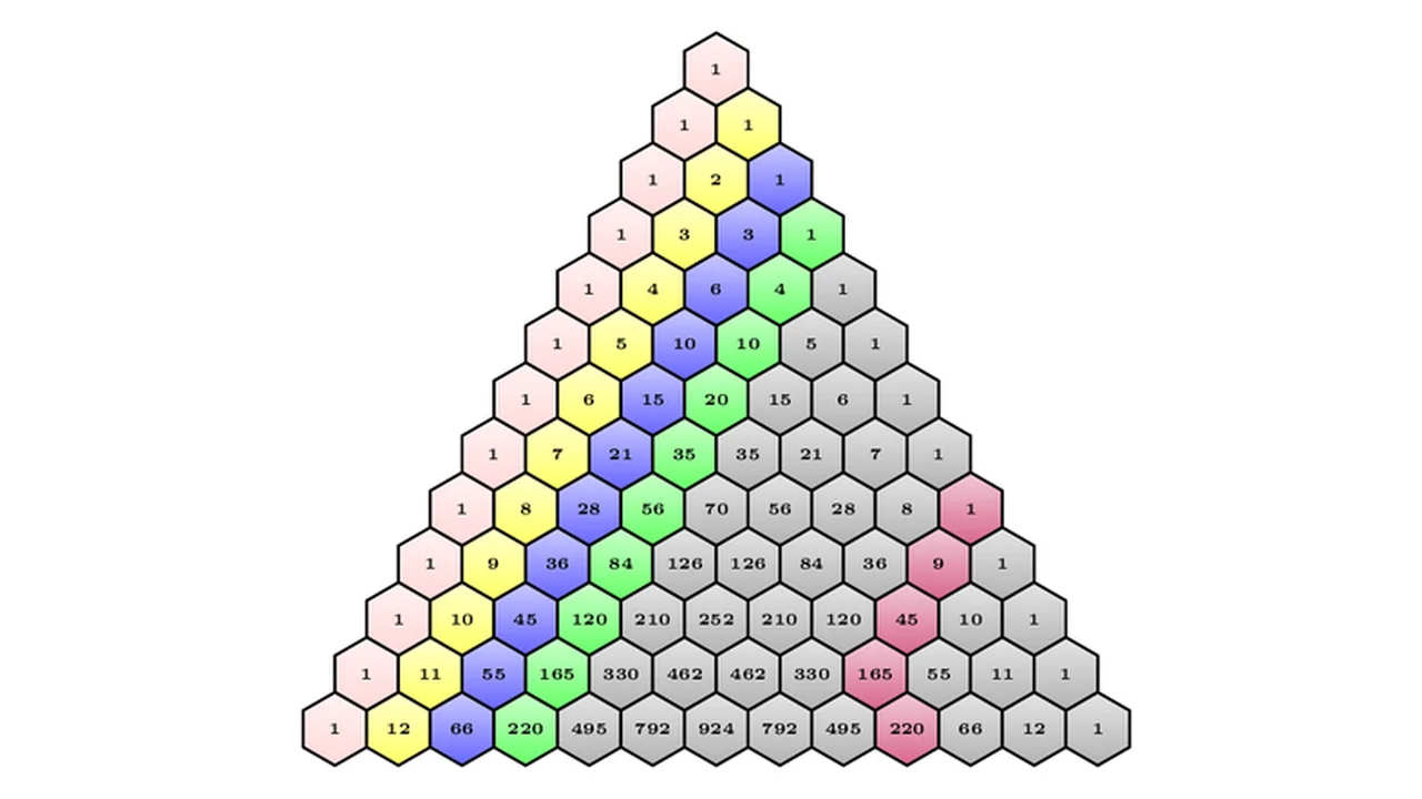
Pascal’s Triangle is a well-known triangular array of binomial coefficients in mathematics. Each number in the triangle is the sum of the two numbers directly above it. In addition to its usefulness in expanding algebraic expressions like $(a+b)^n$, this structure hosts many intriguing patterns.

In this article, we will build a visualization of Pascal’s Triangle in LaTeX using TikZ. Instead of writing the numbers manually, we will leverage TeX macro programming to compute the binomial coefficients dynamically and render them within colorful hexagonal (honeycomb) cells.

Introduction

Geometrically, a honeycomb layout (hexagonal tiling) is ideal for drawing Pascal’s Triangle since each hexagonal cell naturally borders two cells directly above it.

To implement this efficiently in LaTeX, we require two key elements:

1. Computational Algorithm: An internal TeX macro to calculate the binomial coefficients $\binom{n}{k} = \frac{n!}{k!(n-k)!}$ dynamically without exceeding TeX compiler memory limits.
2. Graphical Loops: Nested TikZ loops (\foreach) to draw the hexagons and place them at the correct coordinates according to their row and column values.

Complete LaTeX Code

Here is the complete LaTeX code to generate the colored hexagonal Pascal’s Triangle:

% Pascal triangle
% Author: M.H. Ahmadi
\documentclass[border=10pt]{standalone} 
\usepackage[dvipsnames]{xcolor} 
\usepackage{tikz} 
\usepackage{ifthen} 

\makeatletter
% Macro to compute binomial coefficients \binomialCoefficient{n}{k}
\newcommand\binomialCoefficient[2]{% 
  % Store values 
  \c@pgf@counta=#1% n 
  \c@pgf@countb=#2% k 
  % 
  % Take advantage of symmetry if k > n - k 
  \c@pgf@countc=\c@pgf@counta% 
  \advance\c@pgf@countc by-\c@pgf@countb% 
  \ifnum\c@pgf@countb>\c@pgf@countc% 
    \c@pgf@countb=\c@pgf@countc% 
  \fi% 
  % 
  % Recursively compute the coefficients 
  \c@pgf@countc=1% holds the result 
  \c@pgf@countd=0% counter 
  \pgfmathloop% formula: c -> c*(n-i)/(i+1) for i=0,...,k-1 
    \ifnum\c@pgf@countd<\c@pgf@countb% 
      \multiply\c@pgf@countc by\c@pgf@counta% 
      \advance\c@pgf@counta by-1% 
      \advance\c@pgf@countd by1% 
      \divide\c@pgf@countc by\c@pgf@countd% 
  \repeatpgfmathloop% 
  \the\c@pgf@countc% print result
} 
\makeatother

\begin{document} 

\newdimen\R 
\R=.4cm % Circumradius of the hexagon
\newcommand\mycolor{gray} 

\begin{tikzpicture}[line width=.8pt] 
% Loop for columns (k) from 0 to 12
\foreach \k in {0,...,12}{ 
  \begin{scope}[shift={(-60:{sqrt(3)*\R*\k})}] 
    \pgfmathtruncatemacro\ystart{12-\k} 
    % Loop for rows (n)
    \foreach \n in {0,...,\ystart}{ 
      \pgfmathtruncatemacro\newn{\n+\k} 
      
      % Dynamic color selection based on columns/rows
      \ifthenelse{\k=0}{\def\mycolor{pink}}{} 
      \ifthenelse{\k=1}{\def\mycolor{yellow}}{} 
      \ifthenelse{\k=2}{\def\mycolor{blue}}{} 
      \ifthenelse{\k=3}{\def\mycolor{green}}{} 
      \ifthenelse{\k=8 \AND \n < 4}{\def\mycolor{purple}}{} 
      \ifthenelse{\k=9 \AND \n = 3}{\def\mycolor{purple}}{} 
      
      \begin{scope}[shift={(-120:{sqrt(3)*\R*\n})}] 
        % Draw hexagons with top/bottom gradient colors
        \draw[top color=\mycolor!20,bottom color=\mycolor!60] 
          (30:\R) \foreach \x in {90,150,...,330} { -- (\x:\R)} -- cycle 
          (90:0) node {\tiny $\mathbf{\binomialCoefficient{\newn}{\k}}$}; 
      \end{scope} 
    } 
  \end{scope} 
} 
\end{tikzpicture} 
\end{document}

The output of the code is as follows:

Detailed Code Explanation

The primary TeX and TikZ coding concepts used in the script are explained below:

1. Low-Level TeX Mathematical Computation (\binomialCoefficient)

Due to TeX’s memory limits, calculating large factorials can easily cause buffer overflows. The calculation is optimized using low-level TeX counters (\c@pgf@counta through \c@pgf@countd) to perform fast and precise multiplication and division operations based on the multiplicative formula:

It also implements the symmetry identity $\binom{n}{k} = \binom{n}{n-k}$ to cut down the iteration loop steps by half, speeding up the overall document compilation time.

2. Drawing Regular Hexagons using Polar Coordinates

Regular hexagons are drawn dynamically using TikZ loops and polar coordinates:

(30:\R) \foreach \x in {90,150,...,330} { -- (\x:\R)} -- cycle

This starts drawing the path at $30^\circ$ with radius $R$, then creates line segments pointing to $90^\circ, 150^\circ, 210^\circ, 270^\circ, 330^\circ$, and finally closes the path automatically (-- cycle) to form a perfect equilateral hexagon.

3. Coordinate Vector Offsets (scope and shift)

To stack the hexagons into a triangular arrangement, we use nested scope shifting coordinates:

• The column index is shifted along the $-60^\circ$ vector by $\sqrt{3} \cdot R \cdot k$: shift={(-60:{sqrt(3)*\R*\k})}
• The row index is shifted along the $-120^\circ$ vector by $\sqrt{3} \cdot R \cdot n$: shift={(-120:{sqrt(3)*\R*\n})} Combining these directional offsets correctly maps each cell to its corresponding slot in the symmetric triangle.

4. Dynamic Coloring (\ifthenelse)

The ifthen package is used to apply different background gradients based on the column index:

• Column 0 is shaded pink.
• Column 1 is shaded yellow.
• Column 2 is shaded blue.
• Column 3 is shaded green.
• Specific cells in the bottom-middle are shaded purple to highlight mathematical structures inside the triangle.

How to Compile the Document

1. Ensure a LaTeX distribution (such as TeX Live, MiKTeX, or Overleaf) is installed.
2. Copy the code above and save it as pascal-triangle.tex.
3. Compile using the pdfLaTeX or XeLaTeX engine.
4. The output page will be cropped to the size of the drawing with a 10pt border due to the standalone document class configuration.

Conclusion

Calculating and drawing Pascal’s Triangle dynamically in TikZ LaTeX shows that LaTeX is more than a typesetting system—it is a complete, powerful programming environment. This technique is highly effective for designing clean, mathematically sound teaching materials and graphics without manual calculation. Happy TeXing!