Drawing a Directed Complete Graph (K16) with TikZ in LaTeX

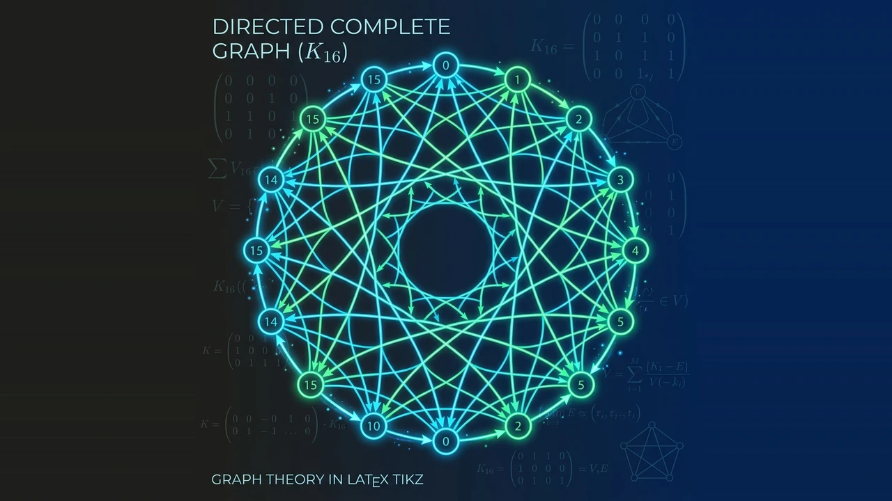
This article explores Graph Theory concepts and LaTeX TikZ coding techniques to render a Directed Complete Graph with 16 nodes ($K_{16}$).

Introduction

In Graph Theory, a complete graph $K_n$ is defined as a simple graph where every pair of distinct vertices is connected by a unique edge.

When extended to a directed complete graph (or symmetric complete digraph), every pair of vertices $u$ and $v$ is connected by two opposing directed edges: one arrow pointing from $u$ to $v$, and another pointing from $v$ to $u$.

This article breaks down a LaTeX TikZ implementation by Quintin Jean-Noël. The code leverages nested loops, TeX counter arithmetic for circular polar positioning, and subtle curved paths (bend left and bend right) to cleanly render 240 directed edges connecting 16 nodes.

Mathematical Analysis: Complete Graph $K_{16}$

For a directed complete graph with $n = 16$ vertices:

1. Number of Vertices ($V$): $|V| = 16$
2. Number of Unique Vertex Pairs: $\binom{16}{2} = \frac{16 \times 15}{2} = 120 \text{ pairs}$
3. Total Directed Edges ($E$): Since each pair has 2 anti-parallel directed edges: $|E| = 2 \times \binom{16}{2} = 16 \times 15 = 240 \text{ directed edges}$
4. Vertex Degree: Each vertex is connected to the remaining 15 vertices:
   • Out-degree: $d^+(v) = 15$
   • In-degree: $d^-(v) = 15$

LaTeX Source Code

Here is the complete TikZ code by Quintin Jean-Noël:

% A complete graph
% Author: Quintin Jean-Noël
\documentclass{article}
\usepackage{tikz}
\usepackage[active,tightpage]{preview}
\PreviewEnvironment{tikzpicture}
\setlength\PreviewBorder{5pt}%
\usetikzlibrary[topaths]

% TeX counter for precise angle calculation
\newcount\mycount

\begin{document}
\begin{tikzpicture}[transform shape]

  % 1. Create First 8 Nodes (Angles: 0, 45, 90, 135, ...)
  \foreach \number in {1,...,8}{
    \mycount=\number
    \advance\mycount by -1
    \multiply\mycount by 45
    \advance\mycount by 0
    \node[draw,circle,inner sep=0.25cm] (N-\number) at (\the\mycount:5.4cm) {};
  }

  % 2. Create Second 8 Nodes with 22.5 Degree Offset (Angles: 22.5, 67.5, ...)
  \foreach \number in {9,...,16}{
    \mycount=\number
    \advance\mycount by -1
    \multiply\mycount by 45
    \advance\mycount by 22.5
    \node[draw,circle,inner sep=0.25cm] (N-\number) at (\the\mycount:5.4cm) {};
  }

  % 3. Connect All Vertex Pairs with Opposing Curved Edges
  \foreach \number in {1,...,15}{
    \mycount=\number
    \advance\mycount by 1
    \foreach \numbera in {\the\mycount,...,16}{
      \path (N-\number) edge[->,bend right=3] (N-\numbera)
                        edge[<-,bend left=3] (N-\numbera);
    }
  }

\end{tikzpicture}
\end{document}

Output Produced

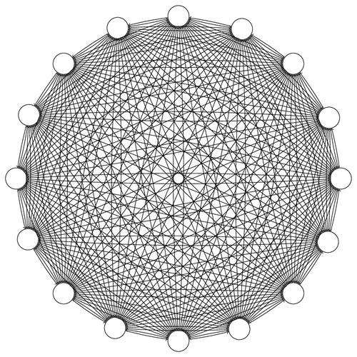
The resulting graphical output displays a dense, symmetrical circular graph network:

Detailed Code Analysis & Logic

1. TeX Counter Arithmetic for Angular Placement

Traditional TeX loops do not support floating-point arithmetic directly inside native loop expressions. To overcome this, the author splits the 16 nodes into two passes using \newcount\mycount:

• Pass 1 (Nodes 1–8): Computes angle $(\text{number} - 1) \times 45^\circ$, producing $0^\circ, 45^\circ, 90^\circ, 135^\circ, 180^\circ, 225^\circ, 270^\circ, 315^\circ$.
• Pass 2 (Nodes 9–16): Adds a $22.5^\circ$ fractional offset, producing $22.5^\circ, 67.5^\circ, 112.5^\circ, 157.5^\circ, 202.5^\circ, 247.5^\circ, 292.5^\circ, 337.5^\circ$.

Each node is assigned a TikZ identifier (N-1) through (N-16) at a radial distance of $5.4\text{ cm}$.

2. Nested Loop Structure

To connect every distinct pair of nodes without duplication:

• The outer loop runs from $i = 1$ to $15$.
• The inner loop runs from $j = i+1$ to $16$.
• This executes exactly $\binom{16}{2} = 120$ iterations.

3. Edge Separation via bend left & bend right

If two opposing directed arrows are drawn as straight lines over each other, they overlap completely and hide directional detail.

• Option edge[->,bend right=3] curves the forward arrow $3^\circ$ to the right.
• Option edge[<-,bend left=3] curves the return arrow $3^\circ$ to the left.
• This subtle curvature creates a small gap between anti-parallel edges, ensuring all 240 directed arrows remain distinctly visible.

TikZ Experimentation

Try these modifications to explore further:

1. Varying Vertex Count ($n$): Try $n = 6$ ($K_6$) or $n = 10$ ($K_{10}$) for a sparser network graph.
2. Distance-Based Edge Coloration: Color edges based on chord length (e.g. blue for adjacent neighbors, red for diameter chords).
3. Bipartite Graph Layout: Arrange nodes in two parallel columns to render a Complete Bipartite Graph ($K_{m,n}$).

Conclusion

Quintin Jean-Noël’s TikZ code provides an excellent example of how abstract Graph Theory objects can be translated into clean visual representations in LaTeX. By leveraging counter calculations and curvature options (bend), 240 directed edges are rendered automatically with precision and balance.

References

1. Quintin Jean-Noël, A complete graph, TeXample.net
2. Till Tantau, The TikZ and PGF Manual, v3.1.10, 2024.
3. Douglas B. West, Introduction to Graph Theory, 2nd Edition, Prentice Hall.

Written by: Aan Triono
License: CC BY-SA 4.0